Predicting eTicketing Revenue with Amazon Forecast

Using Amazon Forecast, an AWS service powered by machine learning, 1CloudHub developed a solution for an eTicketing business focused on transportation tickets to more accurately forecast their revenues. Through improved accuracy, the end customer more accurately predicted their resource requirements, allowing them to reduce their cost structure and increase margins daily.

Use case background

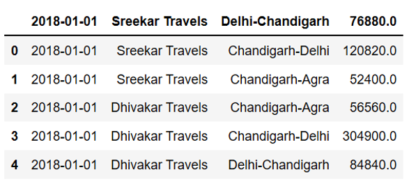
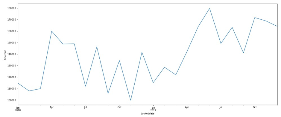
Online Transport’s eTicketing business aggregates thousands of bus operators, each offering transport services across diverse routes vehicles, pickup times, and service levels . Revenues vary widely by operator.  and there is also variability, independent of the operator. For example, revenues are subject to seasonal fluctuations in travel related to weekends, customer demographics, holidays, and other related data.

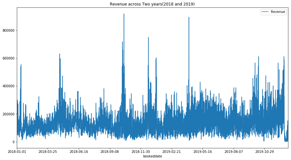
Given the variability in  factors that affect revenues, it is critical for the eTicketing business to develop Sales and Operations processes (S&OP) that allow them to accurately forecast the future daily  from multiple transport operators. Over and under forecasting are both costly mistakes for these mistakes for this business and greater accuracy leads directly to cost efficiency and strategic insights into the revenue performance.

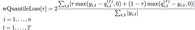
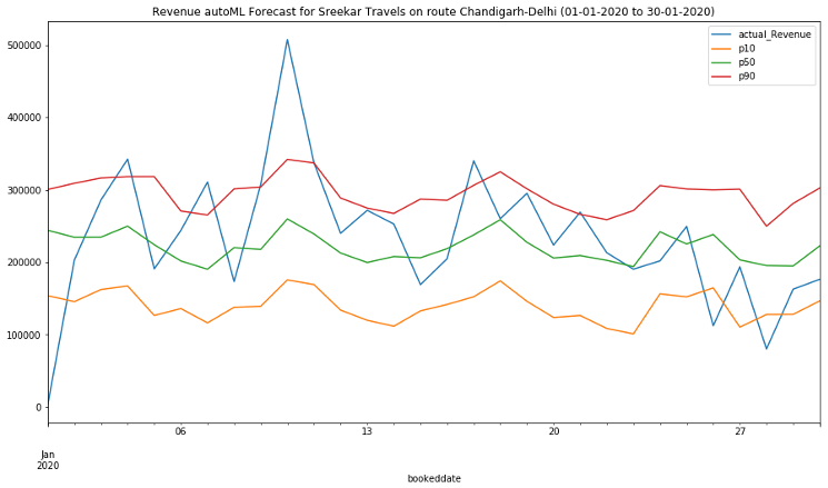
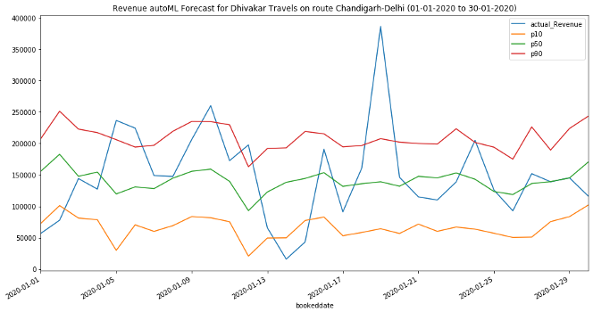
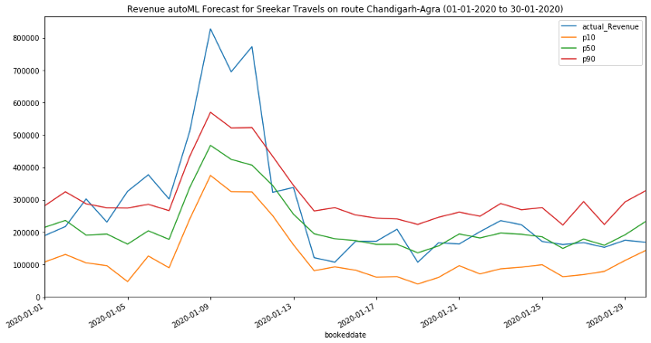
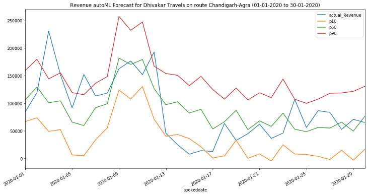
Most other forecasting solutions generate average, point forecasts. However, there is a greater need to factor in uncertainties in the forecasting. This means the forecasts ought to cover not only one possible future but all possible futures which is statistically any quantile value between 1% and 99% denoted as P1 to P99, including mean or the point forecast denoted by P50,with the appropriate weighting according to the probability of a particular outcome. To this end, the key enabler for downstream decision making is a full distribution of the forecast values rather than just having a point forecast., Amazon Forecast generates probabilistic forecasts at a quantile of your choice. In this case, we have considered three default quantiles: 10% (P10), 50% (P50), and 90% (P90). P10 and P90 being under and over forecasts helps quantify the chances of future revenues. Amazon Forecast also allows businesses to define custom quantiles to meet their business needs.

For the P10 forecast, the true value is expected to be lower than the predicted value 10% of the time.

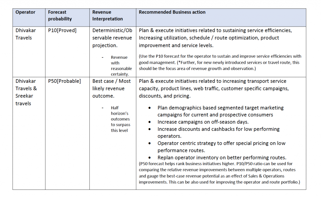
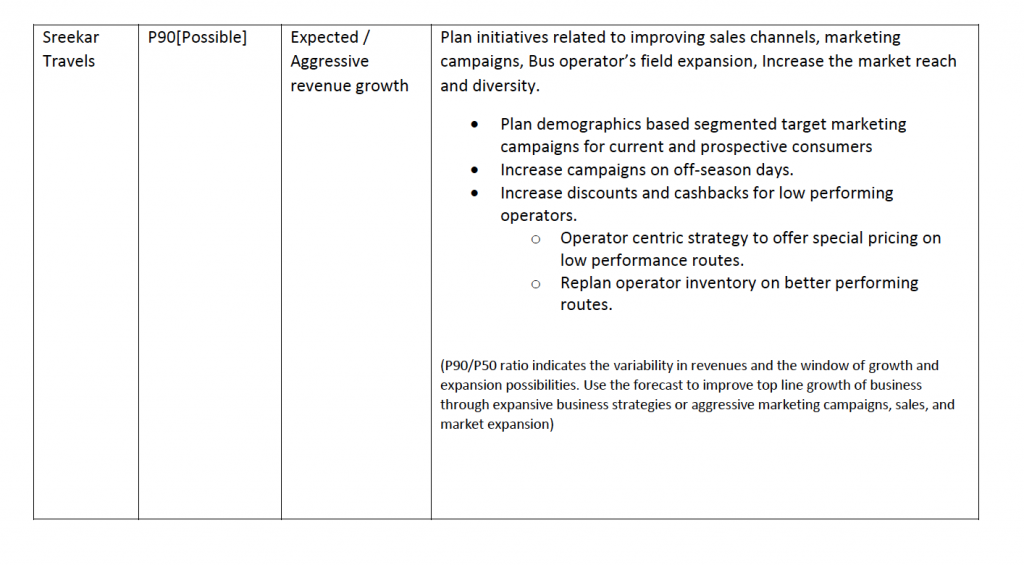
With greater accuracy, deeper insights, and visibility into multiple scenarios through Amazon Forecast, the eTicketing operator could take the following  steps to optimize their marketing and operations to increase the eTicketing revenues.

  • Increase the market campaigns for specific target demographics. For example offering discounts for target customers unlikely to use the service, and loyalty programs for high value customers where churn is costly.
  • Improve e-Ticketing sales by offering incentives to key operator segments, to reduce the drop out ratio in the e-Ticket bookings
  • Improve the visibility of the bus operators with lower forecast revenues in the search page of consumers in the e-ticketing App to improve ticket bookings.
  • Increase the ticket discounts and wallet cashback on the lean days identified in the forecast horizon.
  • Plan a strategy with Bus operators with lower revenues to offer special pricing on identified routes as well as to replan services on profitable routes to improve customer adoption and revenue run rate.

Revenue forecasting scenario

The use case context in our case for an eTicketing transport service aggregator in India involved forecasting revenues for three distinct travel routes of two bus transport operators. The details as follows

  • Operators: – (1) Sreekar Travels, (2) Dhivakar Travels
  • Routes: – (1) Delhi to Chandigarh (2) Chandigarh to Delhi (3) Chandigarh to Agra
  • The forecast horizon was for 30 days (Jan’1 to 30, 2020) based on a Historical time series data for a period of two years available from 01-01-2018 to 31-12-2019 at a daily frequency.

Amazon Forecast Service

Amazon Forecast is a fully managed service that uses machine learning (ML) to generate highly accurate forecasts. In our use case, achieving this required acquiring historical revenue data from multiple transport operators.  Amazon Forecast includes powerful capabilities including support for multiple algorithms. It can automatically load and process the data, select the right algorithms, train a model, provide accuracy metrics, and generate accurate .

Dataset for Forecast Service

For forecasting, we need datasets that contain the timeseries data used to train a predictor. We have to create one or more Amazon Forecast datasets and import the training data into them. A dataset group is a complimentary dataset that detail a set of changing parameters over a series of time.  In a dataset group, Forecast accepts up to three datasets, one of each dataset type which is a) target time series b) related time series, and c) item metadata.    While the target time series data is mandatory requirement, related time series and item meta data are optional based on the availability. After creating a dataset group, it can be used to train a predictor.

Solution Implementation

To use Amazon Forecast, we acquired the historical data pertaining to two bus transport operators combining three travel routes for each operator for forecasting. We had also considered the ticket price as an additional data, also called as related time-series data that we had included in our forecast modelling with the belief that pricing may impact the revenue forecasts.

The historical time series, revenue data acquisition, processing, Model building and Forecast inference was implemented on Amazon Sagemaker as executable notebooks using the Amazon forecast Python SDK. All the data was stored in Amazon S3, a scalable object storage service.

Input

The first steps in using Amazon Forecast are to validate, prepare and import the historical time series data for forecasting.

Amazon Forecast supports the following datasets:

  1. Target Time series, 2. Related Time series, 3.Item Metadata

The target `_id, timestamp, and target value as schema. In our case, we have booked date as timestamp, operator name as item_id and revenue as target value.

You can also add forecast dimension along item_id in forecast. In this case, we have the route as forecast dimension along with operatorname as item_id

The Related time series dataset requires item_id and timestamp. In addition to the required fields, the dataset can include other fields. In our case, we considered ticket price as related series in the data set. You can see this illustrated below in the time series data.

Snapshot of data attributes with target time series (Revenue)
Snapshot of data attributes with related time series (ticket price)

Missing values in input data

A missing value in historical time-series means that the true corresponding value at every period is not available for processing. This needs to be checked for target time series as well as the related time-series and then the data imputation for the forecasting to work properly.

To check missing values in data, we plotted the time series chart as well as used Pandas’ python ‘isnull’ API  as shown below  to visually inspect and numerically check for any missing values in target time series and through this we had confirmed there are were missing values in our data and hence there was no need to impute the data. The data chart and the pandas missing value check output is shown below.

*Please note that an updated version of Amazon forecast now supports automated imputations of missing values (including existing NaNs) for the related and target time series datasets.

With Amazon IAM policies, we can specify allowed or denied actions as well as the conditions under which the resources actions are allowed or denied. This role allows the service to access resources in other services to complete an action on our behalf. We created an IAM Role for Amazon forecast to interact with S3 and Forecast. We setup an IAM role configuration by attaching AmazonForecastFullAccess to access all actions for Amazon Forecast and attaching a ARN policy for the particular S3 bucket to access the target time series data. This IAM role created was used in the Dataset Import job of the target time series.

Algorithms & Approach to Forecast Model Building

Amazon Forecast predictor uses statistical and machine learning algorithms to train a model, then uses the model to make a forecast and it provides the following predefined algorithms viz.,

  1. ARIMA, ETS, NPTS, PROPHET and DeepAR+

To select the Algorithms for modeling, our assumptions included the following

  • The historical time series data would have a seasonal or irregular cycle component. The weekly smoothed revenue chart below mostly suggests that the revenues are cyclic with trends.
  • The monthly smoothed revenues chart in the data also suggested a presence of irregular cycles with some intermittent spiking for multiple times. SMA charts also indicate possible presence of trend components.
  • Presence of noise, the optional variability in the observations
  • Effect of holidays on travel.
  • Normality of distribution of errors
  • Presence of reasonable amount of historical data for each operator, route wise.

Chart: SMA (weekly) of Revenues

Chart: SMA (Monthly) of Revenues

Based on the above assumptions, We took two distinct approaches for forecast modelling (1) Considering only the revenue as the target time series data and (2) Considering ‘ticket price’ as the related time series (RTS) along with the  revenue target series. The RTS price dataset could improve the accuracy of the revenue prediction.

In the first approach we took, our preference for algorithms for building a forecaster with only considering the target time series for modeling were PROPHET, ARIMA and DeepAR+ followed by NPTS and ETS. Our belief was PROPHET algorithm may handle irregular series better along with the holidays and then ARIMA. However, based on the data observations and broader assumptions we had; we took the approach for forecast modeling target time series with all the predefined forecast algorithms available in Amazon Forecast so that we could validate our assumptions and get the relative accuracy of the models. Further, in this, we also leveraged the AutoML capabilities of automatically selecting the best algorithm provided by Amazon Forecast. “PerformAutoML” option made Amazon Forecast to evaluate all algorithms and choose the best algorithm based on our dataset.

In the second approach of forecast modeling with ‘ticket price’ as the related time series, we applied DeepAR+ and PROPHET algorithms that supports RTS.

Forecast Model building

We took the following two approach to build and evaluate the revenue forecast models .

Approach -1 : Data with Target time series

  1. Build Forecast models with “revenue” as the target series using all the algorithms
  2. Apply AutoML to identify the most suitable algorithm as a candidate to baseline. Further, based on the AutoML observations, if the identified algorithm were DeepAR+ , we can apply hyper parameter optimization for tuning .  . .
    • Forecast provides an AutoML option for model training and selection that we will leverage. AutoML automates complex machine learning tasks, for iterative modeling, and model assessment.
  3. Apprach-2: Data with Target time series and Related time seriesBuild Forecast models with “revenue” as the target series and ‘ticket price’ as the related time series (RTS) that is currently supported by PROPHET and DeepAR+ algorithms. The assumption in this second approach was that we expected to see better forecast accuracy as ticket pricing may have a better correlation and influence on the predicted revenues.
  4. Apply AutoML to identify the most suitable algorithm as a candidate to baseline, if the identified algorithm is DeepAR+ , we can apply hyperparameter optimization for tuning.

Finally, we can compare the Approach -1 and 2 outcomes to select a revenue forecast model with a better accuracy.

Further when creating the forecast predictor, we had to set the following parameters.

  • ‘BacktestWindow’ : This is the number of times the algorithm splits the input data for use in training and evaluation and it’s a type of special cross validation.  The config we had set when creating the predictor was 5 (The default value is 1 to 5).
  • ‘BackTestWindowOffset’: We had set this as 100. This is the point in the dataset where we want to split the data for model training and evaluation. Our setting was greater than the forecast horizon of 30 and less than half the length of target time series data which is 2190.
  • Public holiday data for India was enabled

Evaluating Forecast predictor accuracy

Amazon Forecast uses back testing to produce metrics whereby it automatically splits the input data into two datasets, training and test. After the model training, we can get the root mean square error (RMSE) and weighted quantile (wQ) losses to determine how well the model predicted the test data in each back test window and the average value over all the configured five back test windows. These metrics measure the difference between the values predicted by the model and the actual values in the test dataset.

RMSE is the square of the error term, which is the difference between the actual target value, y and the predicted (forecasted) value, ŷ. It is the standard deviation of the residuals (prediction errors). For RMSE, Amazon Forecast uses the P50 forecast to represent the predicted value.

For the probabilistic forecast generated at three quantiles— i.e. P10, P50, and P90, the weighted quantile loss (wQuantileLoss) calculates how far the forecast is from actual demand in either direction as a percentage of demand on average in each quantile. Lower values of ‘wQuantileLoss’ indicate a better overall accuracy of the forecast.

The weighted quantile loss is computed as

where q(tau) is the tau – quantile that the model predicts for tau in the set {0.1, 0.5  0.9}, and y represents the target  series value range in the evaluation period. Amazon Forecast calculates the weighted P10, P50, and P90 quantile losses, where tau is in the set {0.1, 0.5, 0.9}, respectively. These quantiles cover the standard 80% prediction interval region.

Essentially, calculating prediction quantile (intervals) for the model shows how much uncertainty is associated with each forecast. This uncertainty is reflected as the forecast range for the predicted eTicketing revenues. The weighted quantile loss (wQuantileLoss) calculates how far off the forecast is from actual revenues in either direction.    These probabilistic quantiles are explained as below.▪Proved (P10): Revenue projections with reasonable certainty of realization.

  • Indicates there is a 90% chance of realizing revenues at a certain level and with only about a 10% chance that the true revenues may fall below the P10 estimates.


▪Probable (P50):  Revenue projections that is less likely than “Proved” (P10) levels but, more certain to realize than “Possible” (P90) predicted levels.

  • This is the most likely or the best-case revenue. i.e. 50% of the time, revenues would fall above the P50 value, and 50% of the time below the estimate.


▪Possible (P90): Revenue projections less likely to realize than Probable revenue level (P50).

  • In this, there is only a 10% chance of realizing more the P90 forecast level in the given forecast horizon.


It is to be noted that ;

  • P10 forecast overestimates the actual/true Revenues only 10% of the time, so 90% of the time it underestimates the revenues. (the true revenue value is expected to be lower than the predicted P10 only 10% of the time.)
  • P50 forecast overestimates and underestimates revenues 50% of time (e. 50% of the time true revenues are expected to be lower and higher than the P50)
  • P90 forecast overestimates the actual/true revenue 90% of the time. So, 10% of the time, it under-estimates the revenue (the true revenue is expected to be lower than the predicted value 90% of the time.)

Algorithm Selection and Forecast Model metrics

Perform AutoML for Algorithm baselining

As cited in the above mentioned steps, we first used AutoML based modeling to automatically identify the suitable algorithm before making  a production run of the forecasts.

AutoML based Algorithm identification for Target time series

For the target time series modeling using AutoML, DeepAR+ was identified as the baseline algorithm for forecasting as shown below.

AutoML based Algorithm identification with Related time series

For the related timeseries and target timeseries modeling using AutoML, PROPHET was identified as the baseline algorithm for forecasting as shown below..

Forecast Modeling & Selection with baselined algorithms

Based on the AutoML identified algorithms as a baseline, we then built a forecast model pipeline with DeepAR+ with HPO setting enabled for the target time series under approach-1 and with PROPHET for related time series under approach-2 and compared the model performance metrics . Table 1 and 2 below contains the observed RMSE and the weighted quantile loss (wQL) metrics of model evaluation for these predictors. Lower values indicate higher model accuracy.

Final forecast model selection

We finally compare the model metrics for the predictors selected for Approach-1 (DeepAR+) and Approach-2 (PROPHET) which is shown in Table-1 below. As we can observe, the PROPHET forecast model built with Approach-2 using ticket price as the related time series provides a better weighted quantile accuracies with relatively lower error for weighted quantiles wQL[0.9] and and WQL[0.5 ] . These errors are lower than that of DeepAR+ model built with Approach-1.

Further, the RMSE value of PROPHET is also found to be lower in comparison with the DeepAR+ model.  Based on these metrics, we selected PROPHET as the final model for forecasting.

Table #1

Probabilistic Revenue forecasting and Interpretation

After the final model was selected, we queried Amazon forecast to get the probabilistic forecasts for the given horizon of 30 days for Dhivakar and Sreekar travels for the three different routes. While a single point forecast P50 could be used as a simple, single-value revenue forecast, the probabilistic distribution is a better indicator of quantifying uncertainties and possible revenue outcomes in the given forecast horizon. We will use the predicted P10, P50 and P90 forecast distributions or the quantiles   along with its categories that is explained above for the purpose of interpretation.

To interpret the probabilistic forecasts and to illustrate it here, let us investigate the 30-day forecasts for Sreekar and Dhivakar travels pertaining to the Chandigarh-Delhi route and the Chandigarh-Agra route. There are four forecast plots shown below.

Forecast Chart-1 and 2 below shows the P10, P50, P90 probabilistic revenue forecasts of Chandigarh-Delhi route for the two operators as well as the actual / true value of revenues for a horizon of 30 days. X-axis

Forecast Chart-1

Forecast Chart-2

Forecast Chart-3 and 4 below shows the P10, P50, P90 probabilistic revenue forecasts of Chandigarh-Agra route for the two operators as well as the actual / true value of revenues for a horizon of 30 days.

Forecast Chart-3

Forecast Chart- 4

Probabilistic forecast charts above indicate the following:

  • P10 forecast levels indicates revenues with some certainty. As you can see, the true revenue values are found to be above the (P10 – Proved) predicted values almost 90% of the time.
  • Revenues at P90 levels are Possible but are less likely to be realized than revenues at P50 levels and further that revenues at P50 levels “Probable” meaning the chances are most likely realizable at 50% of the time.
  • In comparison to the revenues of the Chandigarh-Delhi route, Chandigarh to Agra route for Dhivakar travels has lower revenue and growth prospects and at the same time, in this Chandigarh to Agra route Sreekar travels seems to be better positioned and competing well.

Deterministic revenues of a Transport operator (Observable Revenue growth)

To decipher further, PP10(Proved) forecast indicates a deterministic revenue level that can be observable in if the current state of business, operations and consumer interests are sustained.

Based on the plots described above, if we compare the PP10 forecast revenues of Sreekar travels with Dhivakar travels for the same travel route (revenue indicated in y-axis of  chart), i.e. Chandigarh to Delhi, forecast revenues at P10 levels is slightly at a higher level than the other. This indicates that Sreekar travels would be able to realize future revenues with reasonable certainty at a level higher than Dhivakar travels.

Best case revenues of a Transport operator (Most likely growth)

P50 forecast indicates probable, best case revenues if the ongoing, current initiatives works well.  The P50 forecast (Probable) provides revenue projections that has a lesser certainty than the P10(proved) level over the forecast horizon but, more certain to realize than “Possible” (P90) predicted revenue levels. If we look at the forecast charts, it indicates Sreekar travels over both the travel routes to potentially realise a higher revenue.

Aggressive Revenues (Expected Growth)

P90 forecast indicates revenues that may be possible through expansionist initiatives combined with operational effectiveness.

The PP90 (Possible) forecast in the horizon for Sreekar travels is slightly at a higher level than Dhivakar travels. This indicates Sreekar travels for the same route has a possibility to grow the revenues at higher levels than Dhivakar travels. This can be considered as an expected revenue growth or a window of opportunity to grow revenues is relatively higher and better.

Probabilistic Forecast Ratios

We can also use the ratios of forecast quantiles to gain insights as the shape of distribution of probabilistic futures can vary. In our case, we consider the following.,

  • P90/P50 ratio: This ratio from the forecast values could be used to assess the variability in revenues. Higher the ratio, higher the spread or dispersion. From a business perspective, this means, more initiatives and efforts may be required to realize revenue potential at a higher level as well as this may require active risk management to reduce uncertainties.
  • P10/P50 ratio: This ratio (tends towards 1 from 0) could be used to assess the quality of observable revenues cited above. A higher ratio suggests better fundamentals in play and a higher level of deterministic revenues. This can be used as a standardized unit to compare and benchmark other bus operators and routes. For instance, we could say all routes with this forecast ratio >=0.75 may be graded as mature and higher quality to generate revenues with higher certainty at than others at a relatively lower level.


Revenue Forecast: key findings and recommendations

  • Revenue Forecast Model: Revenue forecasting with Approach #2 using the PROPHET  model with related time series data provides a forecast with higher for forecasting.
  • Revenue Forecast findings: The observable / deterministic revenue prospects as well as the Best case and Growth of revenues are found to be at a higher level for Sreekar travels when compared against Dhivakar travels for the three travel routes considered in the use case.
  • Forecast based recommendations: Based on the observations from probabilistic forecasts, we provide the following recommendations to Sreekar and Dhivakar travels which includes strengthening and improving operator revenue growth from the perspective of efficiencies, management  to raising the levels of top-line growth, through scaling marketing campaigns and sales expansion. The recommendations are provided in the table given below.

For this online eTicketing business revenue forecast case study, it is important to keep in mind that the forecasting problem is a means to achieving better revenue outcomes. Although the revenue forecasts are crucially important, the Sales, Marketing & Operational decisions are what is even more important. To this end, the key enabler for downstream decision making is a P10,P50 and P90 distribution of the forecast values rather than just having a point forecast and these results assist in understanding the revenue possibilities the eTicketing operator can expect and the related Sales, Marketing and Operations decisions. To Summarize again,

  • Identification or Benchmarking of operators and travel routes by quality of revenues that can lead to a better transport operator and routes portfolio optimization.
  • Prioritizing operational decisions for improving operator-route utilization, service levels and customer engagement and loyalty that can lead to healthy conversions and bottom-line growth.
  • Strategic and tactical decisions pertaining to Sales and Marketing channels, Advt. campaigns, Consumer visibility and reach, New products and services addition and New market expansion that can be aggressively undertaken to improve the growth, sales funnel and raise the top-line growt

We know it has been a long post, but if you followed this blog, it was quite an exciting business use case where Amazon forecast service can be applied to address a high quality, high value business problems that online eTicketing business encounter around aligning revenue forecasting with Sales & Operations improvements and growth respectively.

Thank you for reading and happy Revenue Forecasting!


Financial Forecasting

Written by,


Sankar Nagarajan, Dhivakar Sathya,  Sreekar  & Umashankar N

Sharing is caring!

In Blog
Subscribe to our Newsletter1CloudHub